Network models have become a popular way to abstract complex systems and gain insights into relational patterns among observed variables in many areas of science. The majority of these applications focuses on analyzing the structure of the network. However, if the network is not directly observed (Alice and Bob are friends) but estimated from data (there is a relation between smoking and cancer), we can analyze - in addition to the network structure - the predictability of the nodes in the network. That is, we would like to know: how well can a given node in the network predicted by all remaining nodes in the network?

Predictability is interesting for several reasons:

1. It gives us an idea of how practically relevant edges are: if node A is connected to many other nodes but these only explain, let’s say, only 1% of its variance, how interesting are the edges connected to A?
2. We get an indication of how to design an intervention in order to achieve a change in a certain set of nodes and we can estimate how efficient the intervention will be
3. It tells us to which extent different parts of the network are self-determined or determined by other factors that are not included in the network

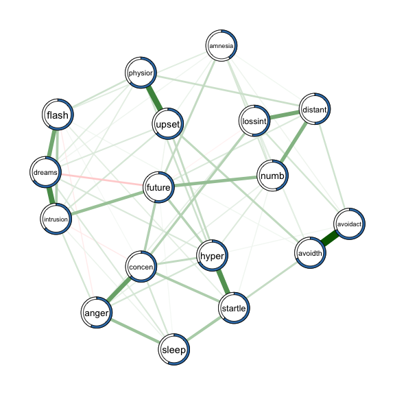
In this blogpost, we use the R-package mgm to estimate a network model and compute node wise predictability measures for a dataset on Post Traumatic Stress Disorder (PTSD) symptoms of Chinese earthquake victims. We visualize the network model and predictability using the qgraph package and discuss how the combination of network model and node wise predictability can be used to design effective interventions on the symptom network.

Load Data

We load the data which the authors made openly available:

data <- read.csv('http://psychosystems.org/wp-content/uploads/2014/10/Wenchuan.csv')
data <- na.omit(data)
data <- as.matrix(data)
p <- ncol(data)
dim(data)

## [1] 344  17

The datasets contains complete responses to 17 PTSD symptoms of 344 individuals. The answer categories for the intensity of symptoms ranges from 1 ‘not at all’ to 5 ‘extremely’. The exact wording of all symptoms is in the paper of McNally and colleagues.

Estimate Network Model

We estimate a Mixed Graphical Model (MGM), where we treat all variables as continuous-Gaussian variables. Hence we set the type of all variables to type = 'g' and the number of categories for each variable to 1, which is the default for continuous variables level = 1:

library(mgm)

set.seed(1)
fit_obj <- mgm(data = data, 
               type = rep('g', p),
               level = rep(1, p),
               lambdaSel = 'CV',
               ruleReg = 'OR', 
               pbar = FALSE)

## Note that the sign of parameter estimates is stored separately; see ?mgm

For more info on how to estimate Mixed Graphical Models using the mgm package see this previous post or the mgm paper.

Compute Predictability of Nodes

After estimating the network model we are ready to compute the predictability for each node. Node wise predictability (or error) can be easily computed, because the graph is estimated by taking each node in turn and regressing all other nodes on it. As a measure for predictability we pick the propotion of explained variance, as it is straight forward to interpret: 0 means the node at hand is not explained at all by other nodes in the nentwork, 1 means perfect prediction. We centered all variables before estimation in order to remove any influence of the intercepts. For a detailed description of how to compute predictions and to choose predictability measures, have a look at this paper. In case there are additional variable types (e.g. categorical) in the network, we can choose an appropriate measure for these variables (e.g. % correct classification, for details see ?predict.mgm).

pred_obj <- predict(object = fit_obj, 
                    data = data, 
                    errorCon = 'R2')

pred_obj$error

##     Variable    R2
## 1  intrusion 0.637
## 2     dreams 0.650
## 3      flash 0.602
## 4      upset 0.637
## 5    physior 0.627
## 6    avoidth 0.686
## 7   avoidact 0.681
## 8    amnesia 0.410
## 9    lossint 0.521
## 10   distant 0.498
## 11      numb 0.458
## 12    future 0.543
## 13     sleep 0.564
## 14     anger 0.561
## 15    concen 0.630
## 16     hyper 0.675
## 17   startle 0.621

We calculated the percentage of explained variance ($R^2$) for each of the nodes in the network. Next, we visualize the estimated network and discuss its structure in relation to explained variance.

Visualize Network & Predictability

We provide the estimated weighted adjacency matrix and the node wise predictability measures as arguments to qgraph() to obtain a network visualization including the predictability measure $R^2$:

library(qgraph)

qgraph(fit_obj$pairwise$wadj, # weighted adjacency matrix as input
       layout = 'spring', 
       pie = pred_obj$error[,2], # provide errors as input
       pieColor = rep('#377EB8',p),
       edge.color = fit_obj$pairwise$edgecolor,
       labels = colnames(data))

The mgm-package also allows to compute predictability for higher-order (or moderated) MGMs and for (mixewd) Vector Autoregressive (VAR) models. For details see this paper. For an early paper looking into the predictability of symptoms of different psychological disorders, see this paper.