Gaussian Mixture Models (GMMs) and its special cases Latent Profile Analysis and k-Means are a popular and versatile tools for exploring heterogeneity in multivariate continuous data. However, they assume that the observed data are continuous, an assumption that is often not met: for example, the severity of symptoms of diseases is often measured in ordinal categories such as not at all, several days, more than half the days, and nearly every day, and survey questions are often assessed using ordinal responses such as strongly agree, agree, neutral, and agree, strongly agree. In this blog post, I summarize a paper which investigates to what extent estimating GMMs is robust against observing ordinal instead of continuous variables.

Simulation Setup

To investigate this question we generate data from a number of GMMs that differ in the number of variables/dimensions $p \in \{2, \dots, 10 \}$, the number of components $K \in \{2,3,4\}$ and the pairwise Kullback-Leibler Divergence $\text{D}_{KL} \in \{2, 3.5, 5\}$ between the components. We then generate data from each GMM and threshold the continuous data into $12, 10, 8, 6, 5, 4, 3,$ or $2$ categories, using equally spaced thresholds ranging from the $0.5\%$ to the $99.5\%$ quantile. The following figure shows the result of this thresholding for a bivariate ($p=2$) GMM with two components ($K=2$):

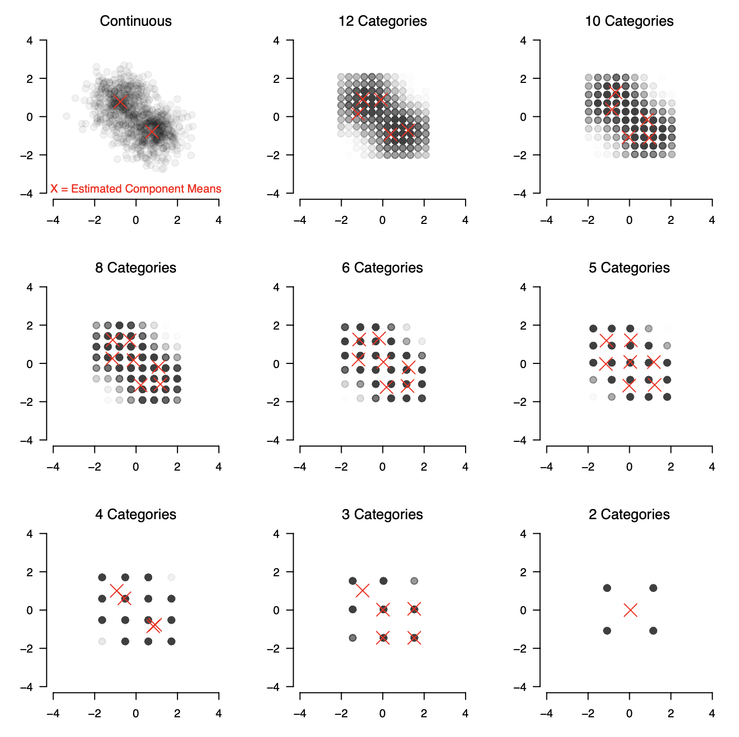
We then estimate the GMM using arguably the most widely used algorithm, the Expectation-Maximization (EM) algorithm and perform model selection with the Bayesian Information Criterion (BIC). The red X in the figure indicate the means of the selected model. We see that the EM-algorithm & BIC correctly recover two components and their means for the continuous data. However, when observing ordinal variables instead we select incorrect numbers of components.

Summary of Results

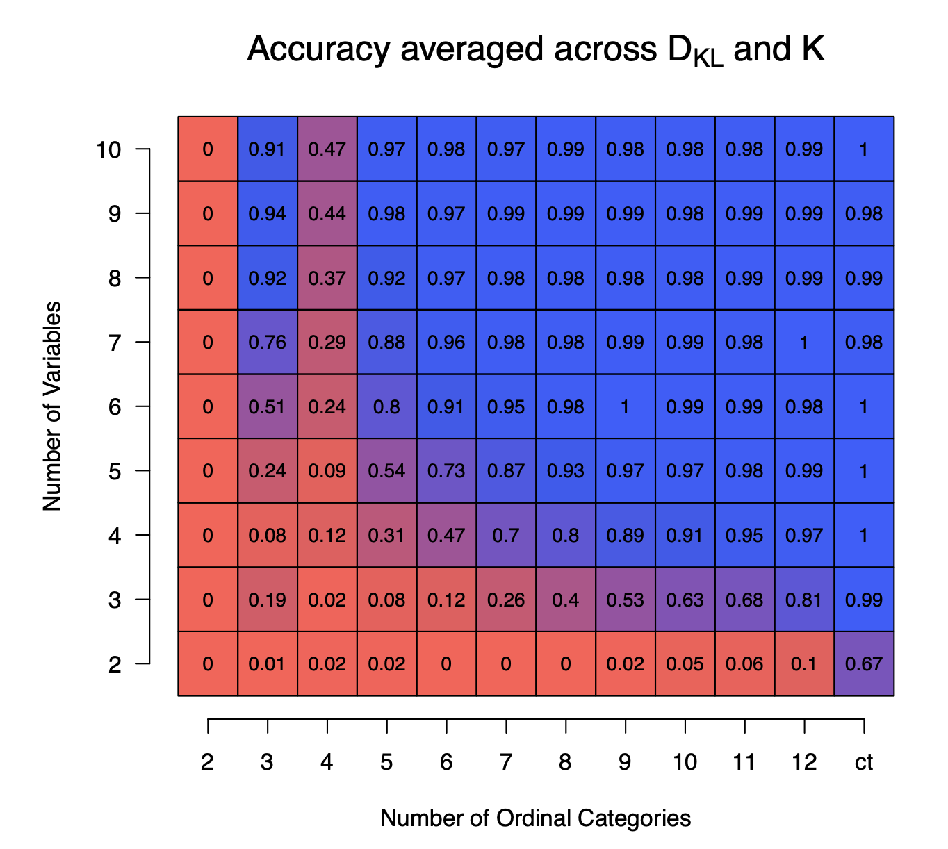
In the following figure we show the accuracy of recovering the correct number of components $K$ averaged across the variations in $K$ and $\text{D}_{KL}$, as a function of the number of variables $p$ (y-axis) and the number of ordinal categories (x-axis) using $N=10000$ samples and averaged across $100$ repetitions. We see that if the number of variables or the number of ordinal categories are low, the accuracy is extremely low. However, when both are larger than $5$ then the accuracy is above $0.90$.

In our paper we present performance as a function of the number of components $K$, the distance between components $\text{D}_{KL}$, the number of variables $p$, and the sample sizes $N \in \{1000, 2500, 10000\}$. In addition, we assess the estimation error on parameters the models for which $K$ has been correctly estimated, as a function of various characteristics of the data generating GMM. These results show that a sizable bias in parameter estimates remains across scenarios and this bias does not decrease with increasing sample size. Next to the simulation results we discuss possible alternative modeling approaches based on ordinal models with underlying latent Gaussian distributions and based on categorical data analysis in which ordinal variables are manifest variables. The code to reproduce all analyses and results in our paper can be found here on Github.