Moderated Network Models for Continuous Data
Statistical network models have become a popular exploratory data analysis tool in psychology and related disciplines that allow to study relations between variables. The most popular models in this emerging literature are the binary-valued Ising model and the multivariate Gaussian distribution for continuous variables, which both model interactions between pairs of variables. In these pairwise models, the interaction between any pair of variables A and B is a constant and therefore does not depend on the values of any of the variables in the model. Put differently, none of the pairwise interactions is moderated. However, in the highly complex and contextualized fields like psychology, such moderation effects are often plausible. In this blog post, I show how to fit, analyze, visualize and assess the stability of Moderated Network Models for continuous data with the R-package mgm.
Moderated Network Models (MNMs) for continuous data are extending the pairwise multivariate Gaussian distribution with moderation effects (3-way interactions). The implementation in the mgm package estimates these MNMs with a nodewise regression approach, and allows one to condition on moderators, visualize the models and assess the stability of its parameter estimates. For a detailed description of how to construct such a MNM, and on how to estimate its parameters, have a look at our paper on MNMs. For a short recap on moderation and its relation to interactions in the regression framework, have a look at this blog post.
Loading & Inspecting the Data
We use a data set with $n=3896$ observations including the variables Hostile, Lonely, Nervous, Sleepy and Depressed, which we took from the 92-item Motivational State Questionnaire (MSQ) data set that comes with the R-package psych. Update June 5 2020: the msq data is not available anymore from the psych package, and we therefore load it manually. Each item is answered on a Likert scale with responses 0 (Not at all), 1 (A little), 2 (Moderately), and 3 (Very much).
data <- read.table("https://jmbh.github.io/files/data/msq.csv", sep=",", header=TRUE)
data <- data[, c("hostile", "lonely", "nervous", "sleepy", "depressed")] # subset
data <- na.omit(data) # exclude rows with missing values

head(data)
## hostile lonely nervous sleepy depressed
## 1 0 1 1 1 0
## 2 0 0 0 1 0
## 3 0 0 0 0 0
## 4 0 1 2 1 1
## 5 0 0 0 1 0
## 6 0 0 0 2 1Because MNMs include next to 2-way (pairwise) interactions also 3-way interactions, they are more sensitive to extreme values. This is because multiplying three of them naturally leads to more extreme values than when multiplying only two extreme values. It is therefore especially important to check the marginal distributions of all variables:
par(mfrow=c(2,3))
for(i in 1:5) {
  barplot(table(data[, i]), axes = FALSE, xlab = "", ylim = c(0, 3000))
  axis(2, las = 2, c(0, 1000, 2000, 3000))
  title(main = colnames(data)[i])
}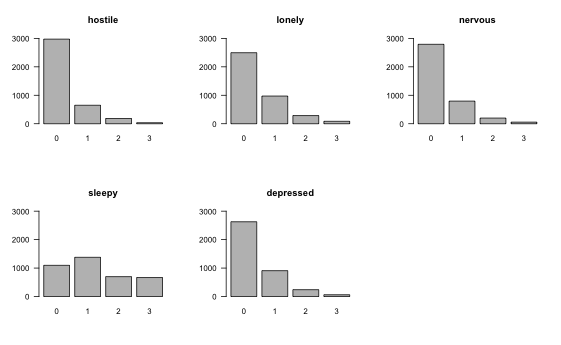
We see that the marginal distributions of all variables except Sleepy are right-skewed and are thereby most likely violating the assumption of MNMs that all variables are conditionally Gaussian. This is the same assumption as in any multiple linear regression model, i.e. that the residuals have a Gaussian distribution. One option would be to transform the variables, possibly by taking the log or square root, or applying the nonparanormal transform. However, any transformation renders the interpretation of parameters more difficult (for example, “increasing X by 1 unit increases the nonparanormal transform of Y by $\beta_{AB}$, keeping everything else constant”), which is why we choose here to use the original variables, but to later check the reliability of our estimates using bootstrapping.
Estimating Moderated Network Model
MNMs can be estimated with the mgm() function, and which moderation effects are included is specified with the moderators argument:
library(mgm) # 1.1-7

set.seed(1)
mgm_mod <- mgm(data = data,
               type = rep("g", 5),
               level = rep(1, 5),
               lambdaSel = "CV",
               ruleReg = "AND",
               moderators = 5,
               threshold = "none",
               pbar = FALSE)
## Note that the sign of parameter estimates is stored separately; see ?mgmOne can specify a particular set of moderation effects by providing a $M \times 3$ matrix to the moderators argument which indicates the specific set of 3-way interactions to be included in the model, where $M$ is the number of included moderation effects. If one provides a vector, then all moderation effects involving the specified variables are included. For the present example we include all moderation effects of the variable Depressed by setting moderators = 5 (Depressed is in column 5).
The remaining arguments are standard arguments of mgm(): type indicates the type of each variable, which in our example is continuous for all variables, which is especified with a "g" for “Gaussian”. level indicates the number of categories of a given variable, which is not applicable for continuous variables and set to 1 by convention. lambdaSel="CV" specifies that the regularization parameters in the $\ell_1$-regularized nodewise estimation approach used in mgm() is selected with cross-validation, and threshold = "none" specifies that no additional thresholding should be performed after estimation.
We can inspect the nonzero interaction parameters in the mgm() output object:
mgm_mod$interactions$indicator## [[1]]
## [,1] [,2]
## [1,] 1 2
## [2,] 1 3
## [3,] 1 4
## [4,] 1 5
## [5,] 2 3
## [6,] 2 4
## [7,] 2 5
## [8,] 3 4
## [9,] 3 5
## [10,] 4 5
##
## [[2]]
## [,1] [,2] [,3]
## [1,] 1 2 5
## [2,] 1 3 5
## [3,] 2 4 5
## [4,] 3 4 5We see that we estimated ten pairwise interactions (that is, all possible $\frac{5(5-1)}{2} = 10$ pairwise interactions) and four 3-way interactions or moderation effects. We see that each nonzero 3-way interaction involves variable 5 (Depression), which has to be the case since we only specified Depression as a moderator. The parameter estimates can be retrieved with the showInteraction() function. For example, for the pairwise interaction between variables 1 (Hostile) and 3 (Nervous) can be obtained like this:
showInteraction(object = mgm_mod, int = c(1,3))## Interaction: 1-3
## Weight: 0.1145438
## Sign: 1 (Positive)We can interpret this parameter using the usual linear regression interpretation: when increasing Nervous (Hostile) by 1 unit, Hostile (Nervous) increases by $\approx 0.114$, keeping everything else constant.
Note, however, that variables 1 and 3 are also involved in a 3-way interaction with 5 (Depressed), that is, the pairwise interaction between 1 and 3 is moderated by 5 (Depression). Similarly to above, we can retrieve the moderation effect using showInteraction():
showInteraction(object = mgm_mod, int = c(1,3,5))## Interaction: 1-3-5
## Weight: 0.05279001
## Sign: 1 (Positive)We see that there is a positive moderation effect. This means that, if one increases the values of Depression, the pairwise interaction between Hostile and Nervous becomes stronger. For example, if Depression = 0, then the parameter for the pairwise interaction between Hostile and Nervous is equal to $0.114 + 0.053 \times 0 = 0.114$. If Depression = 1, then the pairwise interaction parameter is equal to $0.114 + 0.053 \times 1 = 0.167$. In this example, we fixed Depression to a given value and computed the resulting pairwise interaction between Hostile and Nervous We can also do this for the entire network, and inspect the network for different values of Depression. The function condition() does that for you (see below). The discussion of the modereation effect shows that we have to correct our above interpretation of the pairwise interaction between Hostile and Nervous: when increasing Nervous (Hostile) by 1 unit, Hostile (Nervous) increases by $\approx 0.114$, if Depression is equal to zero and when keeping everything else constant.
Why does the pairwise effect represent exactly the effect when Depression is equal to zero? The reason is that we mean-centered all variables before estimation by default. This leads to the situation that the pairwise interaction parameter represents the moderated effect when conditioning on the moderator value with the highest density (assuming that the moderator variable is symmetric and unimodel, which we do here because we assume all variables to be conditional Gaussians). Uncentered variables often lead to pairwise parameters that are conditioned on moderator values that do not exist in the data, which leads to pairwise parameters that have no meaningful interpretation. For a detailed discussion of this see here.
Conditioning on the Moderator
The function condition conditions on (fixes values of) a set of moderators. In our model, we included only a single moderator (Depression), so we only fix the values of Depression. Note that internally, mgm() scales all variables to mean = 0, SD = 1, to ensure that the regularization on parameters does not depend on the variance of the associated variable(s). We therefore need to specify values based on the scaled version of the Depression variable. To pick a reasonable set of values, we inspect the scaled version of the Depression variable:
tb <- table(scale(data$depressed))
names(tb) <- round(as.numeric(names(tb)), 2)
barplot(tb, axes=FALSE, xlab="", ylim=c(0, 3000))
axis(2, las=2, c(0, 1000, 2000, 3000))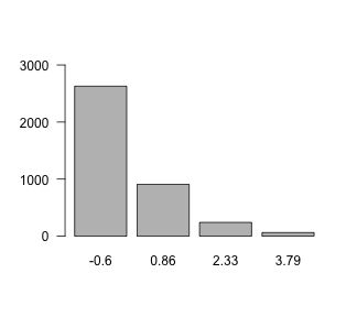
Here, we choose the values 0, 1 and 2.
To condition on, that is, fix a set of variables we provide two arguments to condition(): first, the mgm() output object; and second, a list in which the entry name indicates the variable (by its column number) and the entry value indicates the value to which the variable should be fixed. For example, if we would like to fix Depression = 2 we specify values = list('5' = 2). Here, we call the condition() and fix Depression (5) to the values 0, 1 and 2.
cond0 <- condition(object = mgm_mod,
                   values = list('5' = 0))

cond1 <- condition(object = mgm_mod,
                   values = list('5' = 1))

cond2 <- condition(object = mgm_mod,
                   values = list('5' = 2))
The output of condition() is a complete mgm model object, conditioned on the provided set of variables. For example, cond0 contains the model object conditioned on Depression = 0. On the population level (i.e. if sample size does not play a role), this is the model one would obtain if one took only the rows in which Depression = 0 in the data set, and estimated a pairwise model on this subset of the data.
Note that we can compute the model object conditioned on any value. However, if we specify values that we do not actually observe, for example Depression = 7, we extrapolate beyond the observed data and therefore do not know whether the computed conditional mgm object is accurate.
Since we only specified a single moderator in the present example, the three conditional mgm objects are now pairwise models. We can inspect their parameters as usual, or visualize them:
l_cond <- list(cond0, cond1, cond2)

library(qgraph)
par(mfrow=c(1,3))

max_val <- max(max(l_cond[[1]]$pairwise$wadj),
               max(l_cond[[2]]$pairwise$wadj),
               max(l_cond[[3]]$pairwise$wadj))

for(i in 1:3) qgraph(l_cond[[i]]$pairwise$wadj, layout="circle",
                     edge.color=l_cond[[i]]$pairwise$edgecolor,
                     labels = colnames(msq_p5),
                     maximum = max_val,
                     edge.labels = TRUE, edge.label.cex=2,
                     vsize=20, esize=18,
                     title = paste0("Depression = ", (0:2)[i]))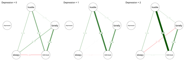
Let’s focus again on the pairwise interaction between Hostile and Nervous. As illustrated above, the relationship becomes stronger when increasing Depression. We also see changes in the three other pairwise interactions that are moderated by Depression: Hostile-Lonely, Lonely-Sleepy, and Nervous-Sleepy. All these conditional pairwise effects can be interpreted as partial correlations. However, note that the pairwise interaction between Hostile-Nervous for Depression=1 computed above ($.167$) is not the same as the one shown in the network picture ($.18$). The reason is that showInteraction() reports the moderation effect aggregated over the estimates of this parameters from all three regressions, while condition() reports the moderation effect aggregated over the two regressions on the two variables in the pairwise interaction. For details have a look at our paper on Moderated Network Models.
Note that Depression is not connected to any other variable in all of the networks. The reason is that in each of the networks Depression is fixed to a value, and therefore technically not part of the model anymore. However, in mgm we keep the variable in the fit object to avoid confusion when comparing MNMs with pairwise models.
Displaying the pairwise networks after conditioning on different values of the moderator variable is perhaps the most intuitive way to report the results of a Moderated Network Model. However, this is only feasible if the number of moderators is small, because the number of cases to consider is equal to $3^m$ if we consider three values for each moderator and have $m$ moderators. In our case we had $3^1=3$ which is still easy to visualize. However, $m=2,3,4$ moderators lead to $9, 27, 81$ cases. An alternative way to visualize MNMs that also works for larger number of moderators is to visualize the MNM in a factor graph.
Visualization using Factor Graph
Here we show how to visualize a MNM that includes several moderators. To this end, we fit the same model as above, but now include all variables as moderators:
set.seed(1)
mgm_mod_all <- mgm(data = data,
                   type = rep("g", 5),
                   level = rep(1, 5),
                   lambdaSel = "CV",
                   ruleReg = "AND",
                   moderators = 1:5,
                   threshold = "none",
                   pbar = FALSE)
## Note that the sign of parameter estimates is stored separately; see ?mgmWe again check which interactions have been estimated to be nonzero
mgm_mod_all$interactions$indicator## [[1]]
## [,1] [,2]
## [1,] 1 2
## [2,] 1 3
## [3,] 1 4
## [4,] 1 5
## [5,] 2 3
## [6,] 2 4
## [7,] 2 5
## [8,] 3 4
## [9,] 3 5
## [10,] 4 5
##
## [[2]]
## [,1] [,2] [,3]
## [1,] 1 2 3
## [2,] 1 2 4
## [3,] 1 3 4
## [4,] 1 3 5
## [5,] 2 3 4
## [6,] 2 4 5
## [7,] 3 4 5and we see that we recovered a few additional 3-way interactions (moderation effects).
Before visualizing this model as a factor graph, let’s consider why we actually need to go beyond a typical network. For example, if there is a 3-way interaction between variables 1-2-3, one could simply connect those three nodes to indicate the 3-way interaction. The problem with this solution, however, is that we cannot tell from the graph alone anymore whether this triangle comes indeed from a 3-way interaction, or from three 2-way (pairwise) interactions, or even a combination of 2-way and 3-way interactions. We therefore need a more powerful graph.
A factor graph includes, as usual, nodes as variables. But it includes additional variables for interaction parameters. That is, we add an additional (factor) node for each 2-way and 3-way interaction. With an mgm() output object as input, the FactorGraph() function plots the factor graph for us:
FactorGraph(mgm_mod_all,
            labels = colnames(data),
            layout = "circle")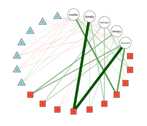
The five round nodes indicate the five variables, while the red square nodes indicate pairwise interactions, and the blue triangle nodes indicate 3-way intereactions. Corresponding to the estimated interactions listed in mgm_mod_all$interactions$indicator we see that there are seven 3-way interactions, and 10 pairwise interactions.
The FactorGraph() function also allows one to only plot 3-way interactions as factor nodes and 2-way interactions as standard edges between variables by setting PairwiseAsEdge = TRUE, which often helps to simply the visualization. In addition, it allows to pass any arguments to qgraph(), which is called by FactorGraph().
Assessing Stability of Estimates
As with pairwise network models, it is useful to obtain a measure for how stable the estimated parameters are. This is especially important in MNMs: first, as discussed at the beginning of this blog post, moderation effects depend more on extreme values than pairwise effects; second, MNMs have more parameters, and therefore the variance on estimates may be larger than for pairwise models; and third, moderation effects are typically smaller than pairwise effects.
To assess stability, we inspect the bootstrapped sampling distributions of all parameters. The function resample() takes the original model object, the data, and the number of bootstrap samples nB as input, and returns an object with nB models fitted on bootstrap samples. Here, we assess the reliability of estimates of the initial example in which Depression was the only moderator (this takes 30-60s to run):
set.seed(1)
res_obj <- resample(object = mgm_mod,
                    data = data,
                    nB = 50,
                    pbar = FALSE)
We can then visualize the summary of all sampling distributions using plotRes():
plotRes(res_obj,
        axis.ticks = c(-.1, 0, .1, .2, .3, .4, .5),
        axis.ticks.mod = c(-.1, -.05, 0, .05, .1),
        cex.label = 1,
        labels = colnames(msq_p5),
        layout.width.labels = .40)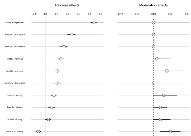
The first column displays the pairwise effects, and the second column shows the moderation effects. The horizontal lines show the 5% and 95% quantiles of the bootstrapped sampling distributions. The number is the proportion of bootstrap samples in which a parameter has been estimated to be nonzero, and the number is placed at the location of the mean of the sampling distribution. We observe that the variance of the sampling distribution is small for pairwise effects, indicating that they are stable.
Regarding the moderation effects, we first notice that moderation effects on pairwise interactions involving Depressed are always zero. Taking the pairwise interaction Lonely-Depressed as an example, the moderation effect would refer to the 3-way interaction Lonely-Depressed-Depressed. Because we do not include such quadratic effects by default, these parameters are always equal to zero. For the moderation effects that were estimated, we see that their mean size are smaller and that the variances are larger relative to their means. However, the moderation effect of Depression on Nervous-Sleepy seems quite stable, and at least the moderation effects on Lonely-Sleepy, and Hostile-Nervous are somewhat stable.
Model Selection
Finally, I would like to address the topic of model selection; specifically, the problem of selecting between models with and without moderation effects. Since all effects are subject to regularization, the model selection in mgm() between models with different regularization parameters essentially selects between models with and without moderation.
An alternative would be to compare the fit of a (possibly unregularized) model including only pairwise interactions with the fit of a (possibly unregularized) model including pairwise interactions and (a set of) moderation effects. This could be done by comparing the fit in a separate training data set, or by approximating out-of-sample error using an out-of-bag error of a cross-validation scheme. These approaches, however, have to be performed on a nodewise basis, because a limitation of MNMs is that it is unclear whether the estimates obtained from nodewise regression give rise to a proper joint distribution. For details see our paper, which precludes using any global likelihood ratio tests or global goodness-of-fit measures. However, all measures can be computed on a nodewise bases and combined to achieve a global model selection.
Moderated Mixed Graphical Models
In the present blog post, I have focused on MNMs that include only continuous variables. However, mgm() also allows one to fit MGMs with moderation effects, in which any type of variable can be a moderator variable that moderates the pairwise interaction between pairs of any types of variables. An interesting special case of this flexible model is a model in which one includes a single categorical variable as a moderator, since this presents an alternative way to estimate group differences between 2 or more groups. I will write a blog post about this in the near future.
Summary
I showed how to estimate Moderated Network Models using mgm() and how to use showInteraction() to retrieve parameter estimates from the output object. For the model including only Depression as a moderator, we used condition() to fix, that is, condition on a set of values of the moderator variable, and used the qgraph package to visualize the separate conditional network models. We showed how to use FactorGraph() to draw a factor graph of an estimated MNM including more than one moderator, which is useful especially when the model includes several moderator variables. And finally, we used resample() and plotRes() to evaluate the stability of estimates using boostrapping.
In case anything is unclear or if you have any questions or comments, please let me know in the comments!
I would like to thank Fabian Dablander and Matti Heino for their feedback on this blog post.
