Researchers are often interested in comparing statistical network models across groups. For example, Fritz and colleagues compared the relations between resilience factors in a network model for adolescents who did experience childhood adversity to those who did not. Several methods are already available to perform such comparisons. The Network Comparison Test (NCT) performs a permutation test to decide for each parameter whether it differs across two groups. The Fused Graphical Lasso (FGL) uses a lasso penalty to estimate group differences in Gaussian Graphical Models (GGMs). And the BGGM package allows one to test and estimate differences in GGMs in a Bayesian setting. In a recent preprint, I proposed an additional method based on moderation analysis which has the advantage that it can be applied to essentially any network model and at the same time allows for comparisons across more than two groups.

In this blog post I illustrate how to estimate group differences in network models via moderation analysis using the R-package mgm. I show how to estimate a moderated Mixed Graphical Model (MGM) in which the grouping variable serves as a moderator; how to analyze the moderated MGM by conditioning on the moderator; how to visualize the conditional MGMs; and how to assess the stability of group differences.

The Data

The data are automatically loaded with the R-package mgm and can be accessed in the object dataGD. The data set contains 3000 observations, of seven variables $X_1, …, X_7$, where $X_7 \in {1, 2, 3}$ indicates group membership. We have 1000 observations from each group. Note that these variables are of mixed type, with $X_1, X_2, X_4,$ and $X_6$ being continuous and the other variables being categorical.

library(mgm) # version 1.2-10

dim(dataGD)

## [1] 3000    7

head(dataGD)

##          x1     x2 x3     x4 x5     x6 x7
## [1,] -0.136 -0.009  0  0.399  0 -0.137  1
## [2,] -0.041  0.803  1  2.475  2  0.181  1
## [3,]  1.011  0.254  1 -0.194  0  1.329  1
## [4,] -0.158 -1.022  1 -1.587  2 -1.377  1
## [5,] -2.157  1.291  1  0.990  0 -0.018  1
## [6,]  0.499 -0.757  1 -0.941  2  1.099  1

In the Appendix of my preprint, I describe how these data were generated.

Fitting a Moderated MGM

Recall that a standard MGM describes the pairwise relationships between variables of mixed types. In order to detect group differences in the pairwise relationships between variables $X_1, X_2, \dots, X_6$ we fit a moderated MGM with the grouping variable $X_7$ being specified as a categorical moderator:

mgm_obj <- mgm(data = dataGD, 
               type = c("g", "g", "c", "g", "c", "g", "c"), 
               level = c(1, 1, 2, 1, 3, 1, 3), 
               moderators = 7, 
               lambdaSel = "EBIC", 
               lambdaGam = 0.25, 
               ruleReg = "AND", 
               pbar = FALSE)

## Note that the sign of parameter estimates is stored separately; see ?mgm

The argument type indicates the type of variable (“g” for continuous-Gaussian, and “c” for categorical) and level indicates the number of categories of each variable, which is set to 1 by default for continuous variables. The moderators argument specifies that the variable in the $7^{th}$ column is included as a moderator. Since we specified via the type argument that this variable is categorical, it will be treated as a categorical moderator. The remaining arguments specify that the regularization parameters in the $\ell_1$-regularized nodewise regression algorithm used by mgm are selected with the EBIC with a hyperparameter of $\gamma=0.25$ and that estimates are combined across nodewise regressions using the AND-rule.

Conditioning on the Moderator

In order to inspect the pairwise MGMs of the three groups, we need to condition the moderated MGM on the values of the moderator variable, which represent the three groups. This can be done with the function condition(), which takes the moderated MGM object and a list specifying on which values of which variables the model should be conditioned on. Here we only have a single moderator variable ($X_7$) and we condition on each of its values ${1, 2, 3}$ which represent the three groups, and save the three conditional pairwise MGMs in the list object l_mgm_cond:

l_mgm_cond <- list()
for(g in 1:3) l_mgm_cond[[g]] <- condition(object = mgm_obj, 
                                           values = list("7" = g))

Visualizing conditioned MGMs

We can now inspect the pairwise MGM in each group similar to when fitting a standard pairwise MGM (for details see the mgm paper or the other posts in my blog). Here we choose to visualize the strength of dependencies in the three MGMs in a network using the qgraph package. We provide the three conditional mgm-objects as an input and set the maximum argument in qgraph() for each visualization to the maximum parameter across all groups to ensure that the visualizations are comparable.

library(qgraph)

v_max <- rep(NA, 3)
for(g in 1:3) v_max[g] <- max(l_mgm_cond[[g]]$pairwise$wadj)

par(mfrow=c(1, 3))
for(g in 1:3) {
  qgraph(input = l_mgm_cond[[g]]$pairwise$wadj, 
         edge.color = l_mgm_cond[[g]]$pairwise$edgecolor_cb,
         lty = l_mgm_cond[[g]]$pairwise$edge_lty,
         layout = "circle", mar = c(2, 3, 5, 3),
         maximum = max(v_max), vsize = 16, esize = 23, 
         edge.labels  = TRUE, edge.label.cex = 3)
  mtext(text = paste0("Group ", g), line = 2.5)
}

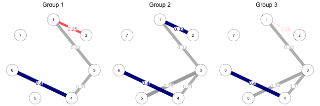
The edges represent conditional dependence relationships and their width is proportional to their strength. The blue (red) edges indicate positive (negative) linear relationships. The grey edges indicate relationships involving categorical variables, for which no sign is defined (for details see ?mgm or the mgm paper). We see that there are conditional dependencies of equal strength between variables $X_1 - X_3$, $X_3 - X_4$ and $X_4 - X_6$ in all three groups. However, the linear dependency between $X_1 - X_2$ differs across groups: it is negative in Group 1, positive in Group 2 and almost absent in Group 3. In addition, there is no dependency between $X_3 - X_5$ in Group 1, but there is a dependency in Groups 2 and 3. Note that the comparable strength in dependencies between those variables in Groups 2 and 3 does not imply that the nature of these dependencies is the same. As with pairwise MGMs, it is possible to inspect the (non-aggregated) parameter estimates of these interactions with the function showInteraction().

Assessing the Stability of Estimates

Similar to pairwise MGMs, we can use the resample() function to assess the stability of all estimated parameters with bootstrapping. Here we only choose 50 bootstrap samples to keep the running time manageable for this tutorial. In practice, the number of bootstrap samples should better be in the order of 1000s.

res_obj <- resample(object = mgm_obj, 
                    data = dataGD, 
                    nB = 50, 
                    pbar = FALSE)

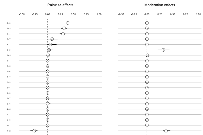
Finally, we can visualize the summaries of the bootstrapped sampling distributions using the function plotRes(). The location of the circles indicates the mean of the sampling distribution, the horizontal lines the 95\% quantiles, and the number in the circle the proportion of estimates that were nonzero.

plotRes(res_obj)

We see that for these simulated data the moderation effects (group differences) are extremely stable. However, note that in observational data moderation effects are typically much smaller and less stable.

Summary

In this blog post, I have shown how to use the mgm-package to estimate a moderated MGM in which the grouping variable serves as a moderator; how to analyze the moderated MNM by conditioning on the moderator; how to visualize the conditional MGMs; and how to assess the stability of group differences. For more details on this method and for a simulation study comparing its performance to the performance of existing methods, have a look at this preprint.

I would like to thank Fabian Dablander for his feedback on this blog post.