Determining conditional independence relationships through undirected graphical models is a key component in the statistical analysis of complex obervational data in a wide variety of disciplines. In many situations one seeks to estimate the underlying graphical model of a dataset that includes variables of different domains.

As an example, take a typical dataset in the social, behavioral and medical sciences, where one is interested in interactions, for example between gender or country (categorical), frequencies of behaviors or experiences (count) and the dose of a drug (continuous). Other examples are Internet-scale marketing data or high-throughput sequencing data.

There are methods available to estimate mixed graphical models from mixed continuous data, however, these usually have two drawbacks: first, there is a possible information loss due to necessary transformations and second, they cannot incorporate (nominal) categorical variables (for an overview see here). When using the recently introduced class of Mixed Graphical Models (MGMs), we avoid these problem because we are able to model each variable on its proper domain.

In the following, we use the R package mgm to estimate a Mixed Graphical Model on a data set consisting of questionnaire responses of individuals diagnosed with Autism Spectrum Disorder. This dataset includes variables of different domains, such as age (continuous), type of housing (categorical) and number of treatments (count).

The dataset consists of responses of 3521 individuals diagnosed with Autism Spectrum Disorder (ASD) to a questionnaire including 28 variables of domains continuous, count and categorical and is automatically loaded with the mgm package.

library(mgm)

dim(autism_data_large$data)

## [1] 3521   28

autism_data_large$data[1:4, 1:5]

##   Gender IQ Age diagnosis Openness about Diagnosis Success selfrating
## 1      1  6    -0.9605781                        1               2.21
## 2      2  6    -0.5156103                        1               6.11
## 3      1  5    -0.7063108                        2               5.62
## 4      1  6    -0.4520435                        1               8.00

We use our knowledge about the variables to specify the domain (type) of each variable and the number of levels for categorical variables (for non-categorical variables we choose 1 by convention). “c”, “g”, “p” stands for categorical, Gaussian and Poisson (count), respectively:

autism_data_large$type

##  [1] "c" "g" "g" "c" "g" "c" "c" "p" "p" "p" "p" "p" "p" "c" "p" "c" "g" "p" "p"
## [20] "p" "p" "g" "g" "g" "g" "g" "c" "g"

autism_data_large$level

##  [1] 2 1 1 2 1 5 3 1 1 1 1 1 1 2 1 4 1 1 1 1 1 1 1 1 1 1 3 1

The mgm-package allows to estimate k-order MGMs (for more details see here). Here we are interested in fitting a pairwise MGM, and we therefore choose k = 2. In order to get a sparse graph, we use L1-penalized regression, which minimizes the negative log likelihood together with the L1 norm of the parameter vector. This penality is weighted by a parameter $\lambda$, which can be selected either using cross validation (lambdaSel = "CV") or an information criterion, such as the Extended Bayesian Information Criterion (EBIC) (lambdaSel = "EBIC"). Here, we choose to use the EBIC with a hyper parameter of $\gamma = 0.25$.

library(mgm)

fit_ADS <- mgm(data = as.matrix(autism_data_large$data), 
               type = autism_data_large$type,
               level = autism_data_large$level,
               k = 2, 
               lambdaSel = 'EBIC', 
               lambdaGam = 0.25, 
               pbar = FALSE)

## Note that the sign of parameter estimates is stored separately; see ?mgm

The fit function returns all estimated parameters and a weighted adjacency matrix. Here we use the qgraph package to visualize the weighted adjacency matrix. The separately provide the edge color for each edge, which indicates the sign of the edge-parmeter, if defined. For more info on the signs of edge-parameters and when they are defined, see the mgm paper or the help file ?mgm. We also provide a grouping of the variables and associated colors, both of which are contained in the data list autism_data_large.

library(qgraph)

qgraph(fit_ADS$pairwise$wadj, 
       layout = 'spring', repulsion = 1.3,
       edge.color = fit_ADS$pairwise$edgecolor, 
       nodeNames = autism_data_large$colnames,
       color = autism_data_large$groups_color, 
       groups = autism_data_large$groups_list,
       legend.mode="style2", legend.cex=.45, 
       vsize = 3.5, esize = 15)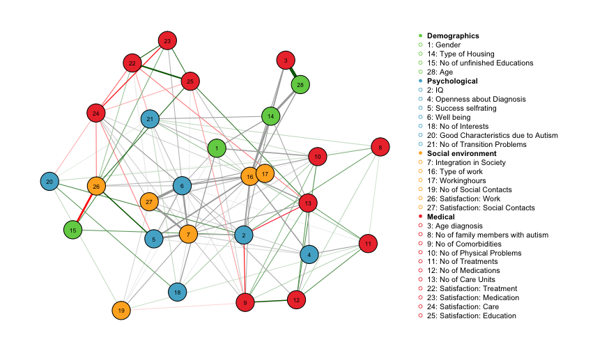

The layout is created using the Fruchterman-Reingold algorithm, which places nodes such that all the edges are of more or less equal length and there are as few crossing edges as possible. Green edges indicate positive relationships, red edges indicate negative relationships and grey edges indicate relationships involving categorical variables for which no sign is defined. The width of the edges is proportional to the absolute value of the edge-parameter. The node color maps to the different domains Demographics, Psychological, Social Environment and Medical.

We observe, for instance, a strong positive relationship between age and age of diagnosis, which makes sense because the two variables are logically connected (one cannot be diagnosed before being born).The negative relationship between number of unfinished educations and satisfaction at work seems plausible, too. Well-being is strongly connected in the graph, with the strongest connections to satisfaction with social contacts and integration in society. These three variables are categorical variables with 5, 3 and 3 categories, respectively. In order to investigate the exact nature of the interaction, one needs to look up all parameters in fit_ADS$rawfactor$indicator and fit_ADS$rawfactor$weights.

For more examples on how to use the mgm package see the helpfiles in the package or the mgm paper. For a tutorial on how to interpret interactions between categorical variables in MGMs see here. For a tutorial on how to compute nodewise predictability in MGMs see here.