Estimating Time-varying Vector Autoregressive (VAR) Models
Models for individual subjects are becoming increasingly popular in psychological research. One reason is that it is difficult to make inferences from between-person data to within-person processes. Another is that time series obtained from individuals are becoming increasingly available due to the ubiquity of mobile devices. The central goal of so-called idiographic modeling is to tap into the within-person dynamics underlying psychological phenomena. With this goal in mind many researchers have set out to analyze the multivariate dependencies in within-person time series. The most simple and most popular model for such dependencies is the first-order Vector Autoregressive (VAR) model, in which each variable at the current time point is predicted by (a linear function of) all variables (including itself) at the previous time point.
A key assumption of the standard VAR model is that its parameter do not change over time. However, often one is interested in exactly such changes over time. For example, one could be interested in relating changes in parameters with other variables, such as changes in a person’s environment. This could be a new job, the seasons, or the impact of a global pandemic. In less exploratory designs, one could examine which impact certain interventions (e.g., medication or therapy) have on the interactions between symptoms.
In this blog post I give a very brief overview of how to estimate a time-varying VAR model with the kernel smoothing approach, which we discussed in this recent tutorial paper. This method is based on the assumption that parameters can change smoothly over time, which means that parameters cannot “jump” from one value to another. I then focus on how to estimate and analyze this type of time-varying VAR models with the R-package mgm.
Estimating time-varying Models via Kernel Smoothing
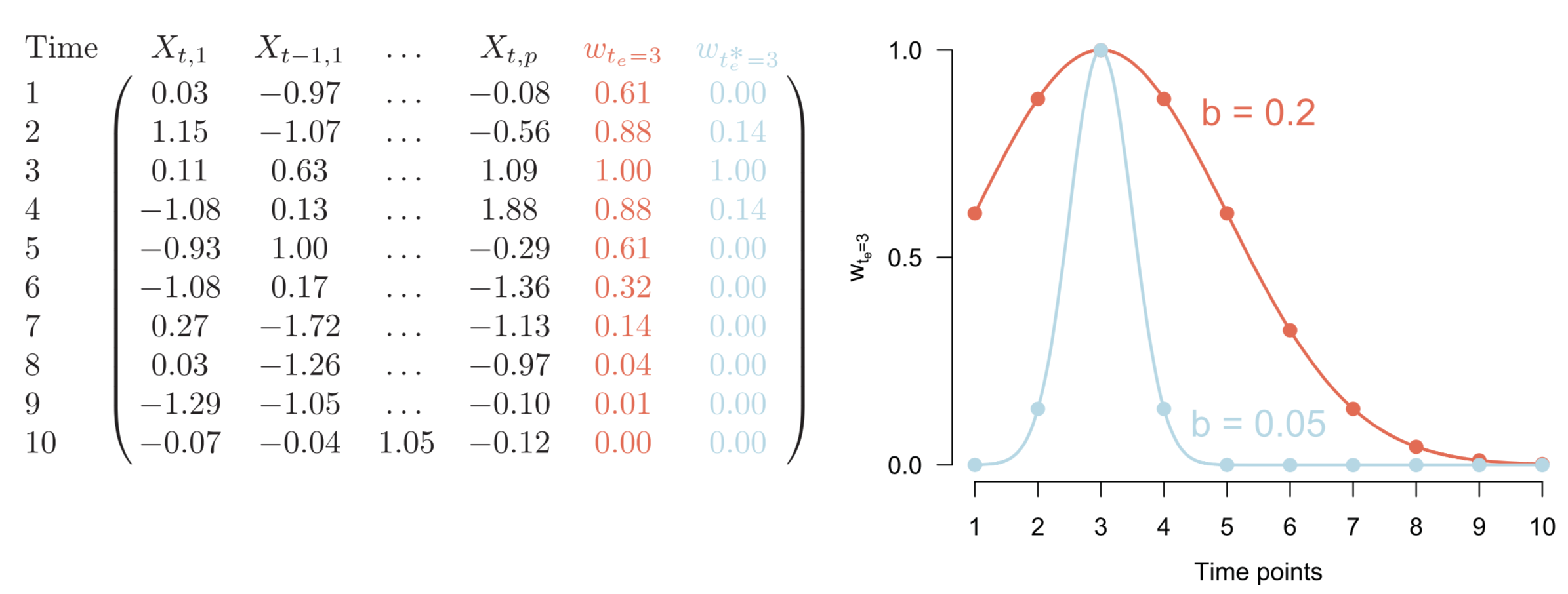
The core idea of the kernel smoothing approach is the following: We choose equally spaced time points across the duration of the whole time series and then estimate “local” models at each of those time points. All local models taken together then constitute the time-varying model. With “local” models we mean that these models are largely based on time points that are close to the time point at hand. This is achieved by weighting observations accordingly during parameter estimation. This idea is illustrated for a toy data set in the following Figure:

Here we only illustrate estimating the local model at $t=3$. We see the 10 time points of this time series on the left panel. The column $w_{t_e=3}$ in red indicates a possible set of weights we could use to estimate the local model at $t=3$: the data at time points close to $t=3$ get the highest weight, and time points further away get an increasingly small weight. The function that defines these weights is shown on the right panel. The blue column in the left panel, and the corresponding blue function on the right indicate another possible weighting. Using this weighting, we combine fewer observations close in time. This allows us to detect more “time-varyingness” in the parameters, because we smooth over less time points. On the other hand, however, we use less data, which makes our estimates less reliable. It is therefore important to choose a weighting function that strikes a good balance between sensitivity to “time-varyingness” and stable estimates. In the method presented here we use a Gaussian weighting function (also called a kernel) which is defined by its standard deviation (or bandwidth). We will return to how to select a good bandwidth parameter below.
In this blog post I focus on how to estimate time-varying models with the R-package mgm. For a more detailed explanation of the method see our recent tutorial paper.
Loading & Inspecting the Data
To illustrate estimating time-varying VAR models, I use an ESM time series of 12 mood related variables that are measured up to 10 times a day for 238 consecutive days (for details about this dataset see Kossakowski et al. (2017)). The questions are “I feel relaxed”, “I feel down”, “I feel irritated”, “I feel satisfied”, “I feel lonely”, “I feel anxious”, “I feel enthusiastic”, “I feel suspicious”, “I feel cheerful”, “I feel guilty”, “I feel indecisive”, and “I feel strong”. Each question is answered on a 7-point Likert scale ranging from “not” to “very”.
The data set is loaded with the mgm-package. We first subset the 12 mood variables:
library(mgm)
mood_data <- as.matrix(symptom_data$data[, 1:12])
mood_labels <- symptom_data$colnames[1:12]
colnames(mood_data) <- mood_labels
time_data <- symptom_data$data_time
We see that the data set has 1476 observations:
dim(mood_data)## [1] 1476 12head(mood_data)## Relaxed Down Irritated Satisfied Lonely Anxious Enthusiastic Suspicious
## [1,] 5 -1 1 5 -1 -1 4 1
## [2,] 4 0 3 3 0 0 3 1
## [3,] 4 0 2 3 0 0 4 1
## [4,] 4 0 1 4 0 0 4 1
## [5,] 4 0 2 4 0 0 4 1
## [6,] 5 0 1 4 0 0 3 1
## Cheerful Guilty Doubt Strong
## [1,] 5 -1 1 5
## [2,] 4 0 1 4
## [3,] 4 0 2 4
## [4,] 4 1 1 4
## [5,] 4 1 2 3
## [6,] 3 1 2 3time_data contains temporal information about each measurement. We will make use of the day on which the measurement occured (dayno), the measurement prompt (beepno) and the overall time stamp (time_norm).
head(time_data)## date dayno beepno beeptime resptime_s resptime_e time_norm
## 1 13/08/12 226 1 08:58 08:58:56 09:00:15 0.000000000
## 2 14/08/12 227 5 14:32 14:32:09 14:33:25 0.005164874
## 3 14/08/12 227 6 16:17 16:17:13 16:23:16 0.005470574
## 4 14/08/12 227 8 18:04 18:04:10 18:06:29 0.005782097
## 5 14/08/12 227 9 20:57 20:58:23 21:00:18 0.006285774
## 6 14/08/12 227 10 21:54 21:54:15 21:56:05 0.006451726Selecting the optimal Bandwidth
One way of selecting a good bandwidth parameter is to fit time-varying models with different candidate bandwidth parameters on a training data set, and evaluate their prediction error on a test data set. The function bwSelect() implements such a bandwith selection scheme. Here we do not show the specification of this function, because it has the same input arguments as the tvmvar() which we describe in a moment below plus a candidate sequence of bandwidth values and some specifications for how to split the data into training and test data. In addition, data driven bandwidth selection can take a considerable amount of time to run, which would not allow you to run the code while reading the blog post. For this tutorial, we therefore just fix the bandwidth to the value that was returned by bwSelect(). However, you can find the code to perform bandwidth selection with bwSelect() on the present data set here).
bandwidth <- .34Estimating time-varying VAR Models
We can now specify the estimation of the time-varying VAR model. We provide the data as input and we specify the type of variables and how many categories they have with the type and level arguments. In our example data sets all variables are continuous, and we therefore set type = rep("g", 12) for continuous-Gaussian, and set the number of categories to 1 by convention. We choose to select the regularization parameters with cross-validation with lambdaSel = "CV", and we specify that the VAR model should include a single lag with lags = 1. The arguments beepvar and dayvar provide the day and the number of notification on a given day for each measurement, which is necessary to specify the VAR design matrix. In addition, we provide the time stamps of all measurements with timepoints = time_data$time_norm to account for missing measurements. Note however, that we still assume a constant lag size of 1. The time stamps are only used to ensure that the weighting indeed gives those time points the highest weight that are closest to the current estimation point (for details see Section 2.5 in this paper). So far, the specification is the same as for the mvar() function which fits stationary mixed VAR models.
For the time-varying model, we need to specify two additional arguments. First, with estpoints = seq(0, 1, length = 20) we specify that we would like to estimate 20 local models across the duration of the entire time series (which is normalized to [0,1]). The number of estimation points can be chosen arbitrarily large, but at some point adding more estimation point is not worth the additional computational costs, because subsequent local models are essentially identical. Finally, we specify the bandwidth with the bandwidth argument.
# Estimate Model on Full Dataset
set.seed(1)
tvvar_obj <- tvmvar(data = mood_data,
                    type = rep("g", 12),
                    level = rep(1, 12),
                    lambdaSel = "CV",
                    lags = 1,
                    beepvar = time_data$beepno,
                    dayvar = time_data$dayno,
                    timepoints = time_data$time_norm,
                    estpoints = seq(0, 1, length = 20),
                    bandwidth = bandwidth,
                    pbar = FALSE)
## Note that the sign of parameter estimates is stored separately; see ?tvmvarWe can paste the output object into the console
# Check on how much data was used
tvvar_obj
## mgm fit-object
##
## Model class: Time-varying mixed Vector Autoregressive (tv-mVAR) model
## Lags: 1
## Rows included in VAR design matrix: 876 / 1476 ( 59.35 %)
## Nodes: 12
## Estimation points: 20which provides a summary of the model and also shows how many rows were in the VAR design matrix (876) compared to the number of time points in the data set (1476). The former number is lower, because a VAR(1) model can only be estimated if for a given time point also the time point 1 lag earlier is available. This is not the case for the first measurement on a given day or if there are missing responses during the day.
Computing Time-varying Prediction Errors
Similarly to stationary VAR models, we can compute prediction errors. This can be done with the predict() function, which takes the model object, the data, and two variables indicating the day number and notification number. Providing the data and the notification variables independently from the model object allows to compute prediction errors for new samples.
The argument errorCon = c("R2", "RMSE") specifies that the proportion of explained variance ($R^2$) and the Root Mean Squared Error (RMSE) should be returned as prediction errors. The final argument tvMethod specifies how time-varying prediction errors should be calculated. The option tvMethod = "closestModel" makes predictions for a time point using the local model that is closest to it. The option chosen here, tvMethod = "weighted", provides a weighted average of the predictions of all local models, weighted using the weighting function centered on the location of the time point at hand. Typically, both methods give very similar results.
pred_obj <- predict(object = tvvar_obj,
                    data = mood_data,
                    beepvar = time_data$beepno,
                    dayvar = time_data$dayno,
                    errorCon = c("R2", "RMSE"),
                    tvMethod = "weighted")
The main output are the following two objects:
pred_obj$tverrors is a list that includes the estimation errors for each estimation point / local model; pred_obj$errors contains the average error across estimation points.
Visualizing parts of the Model
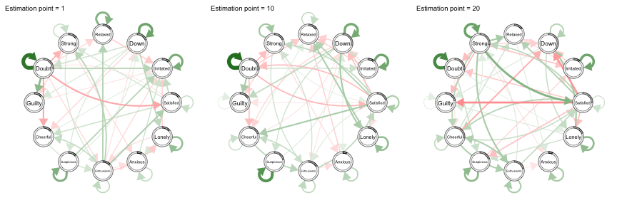
The time-varying VAR(1) model consists of $(p + p^2) \times E$ parameters, where $p$ is the number of variables and $E$ is the number of estimation points. Visualizing all parameters at once is therefore challenging. Instead, one can pick the parameters that are of most interest for the research question at hand. Here, we choose two different visualizations. First, we use the qgraph() function from the R-package qgraph to inspect the VAR interaction parameters at estimation points 1, 10, and 20:
library(qgraph)

par(mfrow=c(1,3))
for(tp in c(1,10,20)) qgraph(t(tvvar_obj$wadj[, , 1, tp]),
                             layout = "circle",
                             edge.color = t(tvvar_obj$edgecolor[, , 1, tp]),
                             labels = mood_labels,
                             mar = rep(5, 4),
                             vsize=14, esize=15, asize=13,
                             maximum = .5,
                             pie = pred_obj$tverrors[[tp]][, 3],
                             title = paste0("Estimation point = ", tp),
                             title.cex=1.2)
dev.off()## null device
## 1We see that some parameters in the VAR models are varying considerably over time. For example, the autocorrelation effect of Relaxed seems to be decreasing over time, the positive effect of Strong on Satisfied only appears at estimation point 20, and also the negative effect of Satisfied on Guilty only appears at estimation point 20.
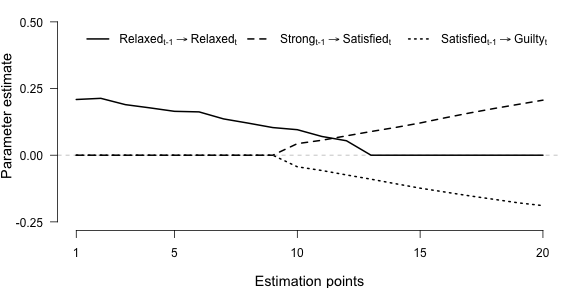
We can zoom in on these individual parameters by plotting them as a function of time:
# Obtain parameter estimates with sign
par_ests <- tvvar_obj$wadj[, , 1, ]
par_ests[tvvar_obj$edgecolor[, , 1, ]=="red"] <- par_ests[tvvar_obj$edgecolor[, , 1, ]=="red"] * -1

# Select three parameters to plot
m_par_display <- matrix(c(1, 1,
                          4, 12,
                          10, 4), ncol = 2, byrow = T)
# Plotting
plot.new()
par(mar = c(4, 4, 0, 1))
plot.window(xlim=c(1, 20), ylim=c(-.25, .55))
axis(1, c(1, 5, 10, 15, 20), labels = T)
axis(2, c(-.25, 0, .25, .5), las = 2)
abline(h = 0, col = "grey", lty = 2)
title(xlab = "Estimation points", cex.lab = 1.2)
title(ylab = "Parameter estimate", cex.lab = 1.2)

for(i in 1:nrow(m_par_display)) {
  par_row <- m_par_display[i, ]
  P1_pointest <- par_ests[par_row[1], par_row[2], ]
  lines(1:20, P1_pointest, lwd = 2, lty = i)
}

legend_labels <- c(expression("Relaxed"["t-1"]  %->%  "Relaxed"["t"]),
                   expression("Strong"["t-1"]  %->%  "Satisfied"["t"]),
                   expression("Satisfied"["t-1"]  %->%  "Guilty"["t"]))
legend(1, .49,
       legend_labels,
       lwd = 2, bty = "n", cex = 1, horiz = T, lty = 1:3)
We see that the effect of Relaxed on itself on the next time point is relatively strong at the beginning of the time series, but then decreases towards zero and remains zero from around estimation point 13. The cross-lagged effect of Strong on Satisfied on the next time point is equal to zero until around estimation point 9 but then seems to increase monotonically. Finally, the cross-lagged effect of Satisfied on Guilty is also equal to zero until around estimation point 13 and then decreases monotonically.
Stability of Estimates
Similar to stationary models, one can assess the stability of time-varying parameters using boostrapped sampling distributions. The mgm package allows one to do that with the resample() function. Here you can find code on how to do that for the example in this tutorial.
Time-varying or not?
Clearly, “time-varyingness” is a continuum that goes from stationary to extremely time-varying. However, in some cases it might be necessary to decide whether the parameters of a VAR model are reliably time-varying. To reach such a decision one can use a hypothesis test with the null hypothesis that the model is not time-varying. Here is one way to perform such a hypothesis test: One begins by fitting a stationary VAR model to the data and then repeatedly simulates data from this estimated model. For each of these simulated time series data sets, one computes a pooled prediction error for the time-varying model. The distribution of these prediction errors serves as the sampling distribution of prediction errors under the null hypothesis. Now one can compute the pooled estimation error of the time-varying VAR model on the empirical data and use it as a test-statistic. This test is explained in more detailed here, and the code to implement this test for the data set used in this tutorial can be found here.
Summary
In this blog post, I have shown how to estimate a time-varying VAR model with a kernel smoothing approach, which is based on the assumption that all parameters are a smooth function of time. In addition to estimating the model, we discussed the selection of an appropriate bandwidth parameter, how to compute (time-varying) prediction errors, and how to visualize different aspects of the model. Finally, I provided pointers to code that shows how to assess the stability of estimates via bootstrapping, and how to perform a hypothesis test one can use to select between stationary and time-varying VAR models.
I would like to thank Fabian Dablander for his feedback on this blog post.
