Yesterday, I read ‘Measurement error and the replication crisis’ by Eric Loken and Andrew Gelman, which left me puzzled. The first part of the paper consists of general statements about measurement error. The second part consists of the claim that in the presence of measurement error, we overestimate the true effect when having a small sample size. This sounded wrong enough to ask the authors for their simulation code and spend a couple of hours to figure out what they did in their paper. I am offering a short and a long version.

Edit Feb 17th: After a nice email converstaion with the authors, I now know that they do make their general argument only under the condition of selecting on significance. Their result then trivially follows from the increased variance of the sampling distribution due to adding ‘measurement error’ (see section (3) below). My source of confusion was that they talk about selection on significance in the paper, but then do not select on significance in the two scatter plots, and incorrectly state in the figure title, that they do. The conclusions of this blog post are still valid when making the assumptions in (1), so I leave it online in case somebody finds (parts of) it interesting.

The Short Version

My conclusion is that the authors show the following: If an estimator is biased (here by the presence of measurement error), then the proportion of estimates that overestimate the true effect depends on the variance of the sampling distribution (which depends on $N$). While this is an interesting insight, the authors do not say this clearly anywhere in the paper. Instead, they use formulations that suggest that they refer to the expected value of the estimator, which does not depend on the sample size. To make things worse, they plot the estimates in a way that suggest that the variance of the estimators is equal for N = 50 and N = 3000 and that the effect is driven by a difference in expected value, while the reverse is true.

The Long Version

I try to make an argument for my claims in the ‘short version’ above in 6 steps. (1) We make clear what the claim is the authors make, (2) we define our terminology, (3) we investigate what adding measurement error does on the population level, (4) we see how this influences the characteristics of estimators based on different sample sizes, (5) we summarize our results and (6) get back to the paper.

(1) The exact claim

The authors write ‘In a low-noise setting, the theoretical results of Hausman and others correctly show that measurement error will attenuate co- efficient estimates. But we can demonstrate with a simple exercise that the opposite occurs in the presence of high noise and selection on statistical significance.’ (p. 584/585). From this we can deduce that the authors claim that ‘In a high noise setting, the presence of measurement error and selection on statistical significance leads to an increase in coefficient estimates’. However, the authors do not select on statistical significance in their simulation, hence we also drop this condition and arrive at the claim ‘In a high noise setting, the presence of measurement error leads to an increase in coefficient estimates’.

What this statement means is unclear to me. Under the reasonable assumption that the authors did not make a fundamental mistake, the rest of this blogpost is about finding out what the authors could have meant.

(2) Terminology (for reference)

In the paper, ‘measurement error’, ‘noise’ and ‘variance’ are used interchangeably. Here, with variances we refer to the variances of the dimensions of the bivariate Gaussian distribution, if not stated otherwise. With measurement error we mean another bivariate Gaussian distribution with zero covariance. By a noisy setting, we refer to a situation with a low signal to noise ratio. This is defined relative to another setting, which is less noisy. The signal to noise ratio is a function of $N$ and is related to the variance of the sampling distribution of the estimator. All these things will become clear in sections (3) and (4).

(3) What does ‘adding measurement error’ mean on the population level?

In order to evaluate the above claim with respect to the simulation setup of the authors, we need to know the simulation setup. Fortunately, the authors provided the code in a quick and friendly email.

The authors consider the problem of estimating the covariance of a bivariate Gaussian distribution from a finite number of observations. The bivariate Gaussian distribution has the density

\[f(x_1, x_2) = \frac{1}{\sqrt{(2 \pi)^k | \mathbf{ \Sigma } | }} \exp \bigl \{ - \frac{1}{2} \bigr (x - \mu)^{\top} \mathbf{ \Sigma }^{-1} (x - \mu) \},\]

where in our case the covariance $cov(x_1, x_2) = r > 0$ is some positive value, so the covariance matrix $\Sigma$ has entries:

\[\Sigma = \begin{bmatrix} 1 & r \\[0.3em] r & 1 \end{bmatrix}\]

Note that if we scale both dimensions of the Gaussian to $\mu_1 = \mu_2 = 0$ and $\sigma_1 = \sigma_2 = 1$ the correlation coefficient is equal to the coefficient of the regression of $x_1$ on $x_2$ or vice versa. Thus all results obtained here also extend to the regression coefficient that is refered to in the paper.

Now the authors ‘add measurement error’ to the two variables which consists of independent Gaussian noise with a variance $k > 0$, where $k$ is a constant. Notice that these two variables can also described by a bivariate Gaussian with covariance matrix $\Sigma^{ME}$:

\[\Sigma^{ME} = \begin{bmatrix} k & 0 \\[0.3em] 0 & k \end{bmatrix}\]

Notice that adding ‘measurement error’ as done by the authors is the same as adding these two Gaussians. Addition is a linear transformation and hence the resulting distribution is again a bivariate Gaussian distribution. Indeed, it turns out that the covariance matrix $\Sigma^A$ of the resulting bivariate Gaussian is the sum of the covariance matrices $\Sigma$ and $\Sigma^{ME}$ of the two bivariate Gaussians:

\[\Sigma^A = \begin{bmatrix} 1 & r \\[0.3em] r & 1 \end{bmatrix} + \begin{bmatrix} k & 0 \\[0.3em] 0 & k \end{bmatrix} = \begin{bmatrix} k + 1 & r \\[0.3em] r & k + 1 \end{bmatrix}\]

Now, if we renormalize the variances to get back to a correlation matrix it becomes obvious that adding ‘measurement error’ has to decrease the absolute value of the covariance:

\[\Sigma^{A_{norm}} = \begin{bmatrix} 1 & \frac{r}{k + 1} \\[0.3em] \frac{r}{k + 1} & 1 \end{bmatrix}\]

Note that $k > 0$ and hence $\frac{r}{k + 1} < r$ and hence the absolute value of the covariance is smaller in \Sigma^{A_{norm}} than in $\Sigma$ in the population.

(4) Properties of the Estimator

We now consider the estimate $\hat \sigma_{1,2}$ for the covariance between $x_1$ and $x_2$ in the bivariate Gaussian with covariance matrix $\Sigma^{A_{norm}}$ which is ‘corrupted’ by measurement error. We obtain $\hat \sigma_{1,2}$ via the least squares estimator, which is an unbiased estimator for $\frac{r}{k + 1}$.

What does this mean? This means that by the Central limit theorem, the sampling distribution will be a Gaussian distribution that is centered on the true coefficient, which is $\frac{r}{k + 1}$. Thus, if we take many samples of size $N$ and compute a coefficient estimate on each of them, the mean coefficient will be equal to $\frac{r}{k + 1}$:

\[\mathbb{E} [\hat \sigma_{1,2}] = \lim_{S \rightarrow \infty} \frac{1}{S} \sum_{i=1}^{\infty} \hat \sigma_{1,2}^i = \frac{r}{k + 1}\]

From the fact that the Gaussian density is symmetric and centered on the true effect, it follows that $\hat \sigma_{1,2}$ will equally often under- and overestimate the true effect $\frac{r}{k + 1}$. It is important to stress that this is true, irrespective of the variance of the sampling distribution (which depends on $N$). We illustrate this in the following Figure which shows the empirical sampling distributions from the simulation of the authors:

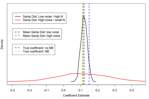
The solid black line indicates the density estimate of the empirical sampling distribution of the coefficient estimates in the low noise (N = 3000) case. The solid red line indicates the density of the empirical sampling distribution of in the high noise (N = 50) case. The dashed black and red lines indicate the arithmetic means of the corresponding sampling distributions. The green dashed line indicates the true coefficient of the bivariate Gaussian with added measurement error. Now, as predicted from the fact that $\hat \sigma_{1,2}$ is an unbiased estimator independent of $N$, we see that the mean parameter estimates in both low/high noise setting (black/red dashed lines) are close to the true coefficient $\frac{r}{k + 1}$ (dashed green line).

Before moving on, we define $\mathcal{P}^\uparrow \in [0,1]$ as the proportion of coefficient estimates that are larger than the true effect $r$ and hence overestimate it. $\mathcal{P}^\uparrow_H$ refers to that proportion in the high noise (small $N$) setting, $\mathcal{P}^\uparrow_L$ refers to that proportion in the low noise (large $N$) setting.

Now, the second important observation is that for both noise settings we have $\mathcal{P}^\uparrow_H = \mathcal{P}^\uparrow_L = \frac{1}{2}$, which implies that we equally often under- and overestimate the true effect. Note that another way of saying this is that the area under the curve left of the green line is equal to the area under the curve right to the orange line, for both sampling distributions.

We now make the crucial step by considering $\hat \sigma_{1,2}$ not as an estimate for the covariance $\frac{r}{k + 1}$ in $\Sigma^{A_{norm}}$, but for the covariance $r$ of the ‘true’ bivariate Gaussian without added measurement error with covariance matrix $\Sigma$. We know that $\hat \sigma_{1,2}$ is an unbiased estimator for $\frac{r}{k + 1}$ and we know $\frac{r}{k + 1} < r$. From this follows that $\hat{\sigma}_{1,2}$ is a biased estimator for $r$. Specifically, the estimator is biased downwards.

We again look at the proportions of coefficient estimates that under- and overestimate the true effect $r$ (the dashed blue line in the figure). We first consider the low noise case: the first observation is that we overestimate $r$ less often than we overestimated $\frac{r}{k + 1}$, which implies $\mathcal{P}^\uparrow_L < \frac{1}{2}$. Again, this is the same as saying that the area under the curve on the right of the blue line is smaller than the area under the curve left to the blue line.

For the high noise case the exact same is true, i.e. $\mathcal{P}^\uparrow_H < \frac{1}{2}$. Let’s define $q := \frac{\mathcal{P}^\uparrow_H}{\mathcal{P}^\uparrow_L}$. Now what we do we have is that $\mathcal{P}^\uparrow_H > \mathcal{P}^\uparrow_L$ and hence $q > 1$. This means that in the presence of measurement error, we overestimate absolutely less often than we underestimate in all settings, however, we overestimate relatively more in a high noise (small $N$) setting compared to a low noise (large $N$) setting. Let’s let this sink in for a moment and then move on to the summary:

(5) Summary

What have we found? We found that if our estimator is biased downwards (here by measurement error), then different sample sizes (and hence different variances of the sampling distribution) lead to different proportions of coefficient estimates that overestimate the true effect.

However, it is important to stress: when keeping $N$ constant and introducing measurement error, the proportion of overestimating estimates decreases compared to the situation without measurement error. This is because the whole sampling distribution is shifted towards zero in the presence of measurement error (the blue line is shifted to the position of the green line in the Figure).

The only thing that is increasing is $q$, which means that in the presence of measurement error in a high noise setting (small $N$) we relatively overestimate more than in a low noise setting (high $N$). What determines $q$? The larger the difference between the variances of two sampling distributions, the larger $q$. The more we shift the sampling distribution towards zero (by adding measurement error), the larger $q$.

(6) Back to the Paper

I think the results stated in (5) are pretty far away from the claim in the paper, which was ‘In a high noise setting, the presence of measurement error leads to an increase in coefficient estimates’. This statement rather suggests that introducing measurement error increases the expected value of the sampling distribution (moving the blue line to the right instead of to the left) which is - as we have seen - incorrect. This false suggestion is strengthened by the scaling of the figures. We illustrate this here, by plotting the figure as shown in the paper (top row) and with equal coordinate systems (bottom row).

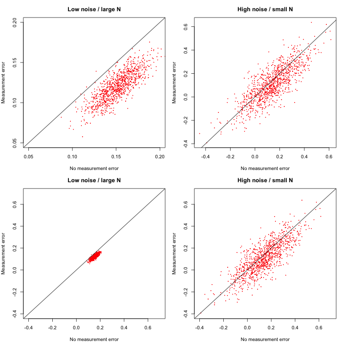
The top row suggests that the difference between the low/high noise setting is because the whole cloud is ‘shifted’ downwards in the low noise setting. This would mean that the sampling distributions are shifted differently depending on the noise setting (sample size) when adding measurement error. On the other hand, when plotting the data in the same coordinate system, it is clear that the expected values do not change and that effect is driven by the differing variances of the estimator.

And one more thing: in the right panel in the figure of the paper the authors plot $\mathcal{P}^\uparrow$ as a function of $N$. Note that from the discussion in (4) it follows that this value can never be larger than $\frac{1}{2}$ as long as the estimator is unbiased or biased downwards. So there must have been some mistake.

Conclusion

This was a fun opportunity to do some statistics detective work. However, the lack of clarity does potentially also do quite some harm by confusing the reader about important concepts. There is of course also the possibility that I just fully misunderstood their paper. In that case I hope the reader will point to my mistakes.

The code to exactly reproduce the above figures can be found here.

I would like to thank Fabian Dablander and Peter Edelsbrunner for helpful comments on this blogpost. In addition, I would like to thank Oisín Ryan and Joris Broere for an interesting discussion on a train ride from Eindhoven to Utrecht yesterday, and I apologize to about 15 anonymous Dutch travelers because they had to endure a heated statistical debate.

I am looking forward to comments, complaints and corrections.